VV in SiC
An example of computing Free Induction Decay (FID) and Hahn-echo (HE) with hyperfine couplings from GIPAW for axial and basal divacancies.
import numpy as np
import matplotlib.pyplot as plt
import sys
import ase
import pandas as pd
import warnings
import pycce as pc

np.set_printoptions(suppress=True, precision=5)
warnings.simplefilter("ignore")

seed = 8805
Axial kk-VV
First we compute FID and HE for axial divacancy.
Build BathCell from the ground
One can set up an BathCell instance by providing the parameters of the unit cell, or cell argument as 3x3 tensor, where each column defines a, b, c unit cell vectors in cartesian coordinates.
In this tutorial we use the first approach.
# Set up unit cell with (a, b, c, alpha, beta, gamma)
sic = pc.BathCell(3.073, 3.073, 10.053, 90, 90, 120, 'deg')
# z axis in cell coordinates
sic.zdir = [0, 0, 1]
Next, user has to define positions of atoms in the unit cell. It is done with BathCell.add_atoms function. It takes an unlimited number of arguments, each argument is a tuple. First element of the tuple is the name of the atom, second - list of xyz coordinates either in cell units (if keyword type='cell', default value) or in Angstrom (if keyword type='angstrom'). Returns BathCell.atoms dictionary, which contains list of coordinates for each type of elements.
# position of atoms
sic.add_atoms(('Si', [0.00000000, 0.00000000, 0.1880]),
              ('Si', [0.00000000, 0.00000000, 0.6880]),
              ('Si', [0.33333333, 0.66666667, 0.4380]),
              ('Si', [0.66666667, 0.33333333, 0.9380]),
              ('C', [0.00000000, 0.00000000, 0.0000]),
              ('C', [0.00000000, 0.00000000, 0.5000]),
              ('C', [0.33333333, 0.66666667, 0.2500]),
              ('C', [0.66666667, 0.33333333, 0.7500]));
Two types of isotopes present in SiC: \(^{29}\)Si and \(^{13}\)C. We add this information with the BathCell.add_isotopes function. The code knows most of the concentrations, so this step is actually unnecessary. If no isotopes is provided, the natural concentration of common magnetic isotopes is assumed.
# isotopes
sic.add_isotopes(('29Si', 0.047), ('13C', 0.011))

# defect position in cell units
vsi_cell = [0, 0, 0.1880]
vc_cell = [0, 0, 0]

# Generate bath spin positions
atoms = sic.gen_supercell(200, remove=[('Si', vsi_cell),
                                       ('C', vc_cell)],
                          seed=seed)
Read Quantum Espresso output
PyCCE provides a helper function read_qe in pycce.io module to read hyperfine couplings from quantum espresso output. read_qe takes from 1 to 3 positional arguments:
pwfilename of the pw input/output file;hyperfinename of the gipaw output file containing hyperfine couplings;efgname of the gipaw output file containing electric field tensor calculations.
During its call, read_qe will read the cell matrix in pw file and apply it to the coordinates is necessary. However, usually we still need to rotate and translate the Quantum Espresso supercell to allign it with our BathArray. To do so we can provide additional keywords arguments center and rotation_matrix. center is the position of (0, 0, 0) point in coordinates of pw file, and rotation_matrix is rotation matrix which aligns z-direction of the GIPAW output. This matrix,
acting on the (0, 0, 1) in Cartesian coordinates of GIPAW output should produce (a, b, c) vector, alligned with zdirection of the BathCell. Keyword argument rm_style shows whether rotation_matrix contains coordinates of new basis set as rows ('row', common in physics) or columns ('col', common in math).
# Prepare rotation matrix to alling with z axis of generated atoms
# This matrix, acting on the [0, 0, 1] in Cartesian coordinates of GIPAW output
# Should produce [a, b, c] vector, alligned with zdirection of the BathCell
M = np.array([[0, 0, -1],
              [0, -1, 0],
              [-1, 0, 0]])

# Position of (0,0,0) point in cell coordinates
center = [0.6, 0.5, 0.5]
# Read GIPAW results
exatoms = pc.read_qe('axial/pw.in',
                     hyperfine='axial/gipaw.out',
                     center=center, rotation_matrix=M,
                     rm_style='col',
                     isotopes={'C':'13C', 'Si':'29Si'})
pc.read_qe produces instance of BathArray, with names of bath spins as the most common isotopes of the following elements (if keyword isotopes set to None) or from the mapping provided by the isotopes argument.
Set up CCE Simulator
In this example we set up a bare Simulator and add properties of the spin bath later.
# Setting up CCE calculations
pos = sic.to_cartesian(vsi_cell)
CCE_order = 2
r_bath = 40
r_dipole = 8
B = np.array([0, 0, 500])

calc = pc.Simulator(1, pos, alpha=[0, 0, 1], beta=[0, 1, 0], magnetic_field=B)
Function Simulator.read_bath can be called explicitly to initiallize spin bath. Additional keyword argument external_bath takes instance of BathArray with hyperfine couplings read from Quantum Espresso. The program then finds the spins with the same name at the same positions (within the range defined by error_range keyword argument) in the total bath and sets their hyperfine couplings.
Finally, we call Simulator.generate_clusters to find the bath spin clusters in the provided bath.
calc.read_bath(atoms, r_bath, external_bath=exatoms);
calc.generate_clusters(CCE_order, r_dipole=r_dipole);
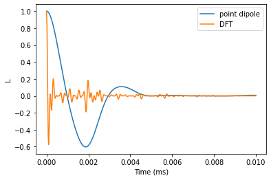
FID with DFT hyperfine couplings
We provide pulses argument directly to the compute function instead of during initiallization of the Simulator object.
time_space = np.linspace(0, 0.01, 501)
N = 0

ldft = calc.compute(time_space, pulses=N, as_delay=False)
FID with hyperfine couplings from point dipole approximation
pdcalc = pc.Simulator(1, pos, alpha=[0, 0, 1], beta=[0, 1, 0], magnetic_field=B,
                      bath=atoms, r_bath=r_bath, order=CCE_order, r_dipole=r_dipole)
lpd = pdcalc.compute(time_space, pulses=N, as_delay=False)
Plot the results and and verify that the predictions are significantly different.
plt.plot(time_space, lpd.real, label='point dipole')
plt.plot(time_space, ldft.real, label='DFT')
plt.legend()
plt.xlabel('Time (ms)')
plt.ylabel('L');
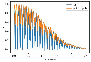
Hahn-echo comparison
Now we compare the predictions for Hahn-echo signal with different hyperfine couplings.
he_time = np.linspace(0, 2.5, 501)
B = np.array([0, 0, 500])
N = 1

he_ldft = calc.compute(he_time, magnetic_field=B, pulses=N, as_delay=False)
he_lpd = pdcalc.compute(he_time, magnetic_field=B, pulses=N, as_delay=False)
Plot the results and compare. We observe that electron spin echo modulations differ significantly, while the observed decay is about the same.
plt.plot(he_time, he_ldft.real, label='DFT')
plt.plot(he_time, he_lpd.real, label='point dipole')

plt.legend()
plt.xlabel('Time (ms)')
plt.ylabel('L');
Basal kh-VV in SiC
The basal divacancy’s Hamiltonian includes both D and E terms, which allows for mixing between +1 and -1 spin levels at zero field.
Thus, either the generalized CCE should be used, or additional perturbational Hamiltonian terms are to be added. Here we consider the generalized CCE framework.
First, prepare rotation matrix for DFT results. The same supercell was used to compute hyperfine couplings, however z-axis of the electron spin qubit is aligned with Si-C bond, therefore we will need to rotate the DFT supercell accordingly.
# Coordinates of vacancies in cell coordinates (note that Vsi is not located in the first unitcell)
vsi_cell = -np.array([1 / 3, 2 / 3, 0.0620])
vc_cell = np.array([0, 0, 0])

sic.zdir = [0, 0, 1]

# Rotation matrix for DFT supercell
R = pc.rotmatrix([0, 0, 1], sic.to_cartesian(vsi_cell - vc_cell))
Total spin bath can be initiallized by simply setting z direction of the BathCell object.
sic.zdir = vsi_cell - vc_cell

# Generate bath spin positions
sic.add_isotopes(('29Si', 0.047), ('13C', 0.011))
atoms = sic.gen_supercell(200, remove=[('Si', vsi_cell),
                                       ('C', vc_cell)],
                          seed=seed)
Read DFT results with read_qe function. To rotate in the correct frame we need to apply both changes of basis consequently
M = np.array([[0, 0, -1],
              [0, -1, 0],
              [-1, 0, 0]])

# Position of (0,0,0) point in cell coordinates
center = np.array([0.59401, 0.50000, 0.50000])

# Read GIPAW results
exatoms = pc.read_qe('basal/pw.in',
                     hyperfine='basal/gipaw.out',
                     center=center, rotation_matrix=(M.T @ R),
                     rm_style='col',
                     isotopes={'C':'13C', 'Si':'29Si'})
To check whether our rotations produced correct results we can find the indexes of the BathArray and DFT output with pc.same_bath_indexes function. It returns a tuple, containing the indexes of elements in the two BathArray instances with the same position and name. First element of the tuple - indexes of first argument, second - of the second. For that we generate supecell with BathCell class, containing 100% isotopes, and count the number of found indexes - iut should be equal
to the size of DFT supercell.
# isotopes
sic.add_isotopes(('29Si', 1), ('13C', 1))
allcell = sic.gen_supercell(50, remove=[('Si', vsi_cell),
                                       ('C', vc_cell)],
                            seed=seed)

indexes, ext_indexes = pc.same_bath_indexes(allcell, exatoms, 0.2, True)
print(f"There are {indexes.size} same elements."
      f" Size of the DFT supercell is {exatoms.size}")
There are 1438 same elements. Size of the DFT supercell is 1438
Setting up calculations
Now we can safely setup calculations of coherence function with DFT couplings. We will compare results with or without bath state sampling.
D = 1.334 * 1e6
E = 0.0184 * 1e6
magnetic_field = 0

calc = pc.Simulator(1, pos, bath=atoms, external_bath=exatoms, D=D, E=E,
                    magnetic_field=magnetic_field, alpha=0, beta=1,
                    r_bath=r_bath, order=CCE_order, r_dipole=r_dipole)
The code automatically picks up the two lowest eigenstates of the central spin hamiltonian as qubit states.
print(calc)
Simulator for center array of size 1.
magnetic field:
array([0., 0., 0.])

Parameters of cluster expansion:
r_bath: 40
r_dipole: 8
order: 2

Bath consists of 761 spins.

Clusters include:
761  clusters of order 1.
1870  clusters of order 2.
We can use the CenterArray, stored in Simulator.center attribute, to take a look at the qubit states in the absence of nuclear spin bath.
calc.center.generate_states()
print(f'0 state: {calc.alpha.real}; 1 state: {calc.beta.real}')
0 state: [ 0. -1. 0.]; 1 state: [ 0.70711 0. -0.70711]
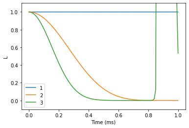
Free Induction Decay (FID)
Now, use the generalized CCE to compute FID of the coherence function at different CCE orders.
N = 0 # Number of pulses
time_space = np.linspace(0, 1, 101) # Time points at which to compute

orders = [1, 2, 3]
lgen = []

r_bath = 30
r_dipole = 8

calc = pc.Simulator(1, pos, bath=atoms, external_bath=exatoms,
                    D=D, E=E, pulses=N, alpha=0, beta=1,
                    r_bath=r_bath, r_dipole=r_dipole)
for o in orders:
    calc.generate_clusters(o)
    l = calc.compute(time_space, method='gcce',
                     quantity='coherence', as_delay=False)

    lgen.append(np.abs(l))

lgen = pd.DataFrame(lgen, columns=time_space, index=orders).T
We see that the results do not converge, but rather start to diverge. Bath sampling (setting nbstates to some value) will help with that.
lgen.plot()
plt.xlabel('Time (ms)')
plt.ylabel('L')
plt.ylim(-0.1, 1.1);
Note, that this approach is nbstates times more expensive than the gCCE, therefore the following calculation will take a couple of minutes.
orders = [1, 2]
lgcce = []

r_bath = 30
r_dipole = 6

for o in orders:
    calc.generate_clusters(o)

    l = calc.compute(time_space, nbstates=30, seed=seed,
                     method='gcce',
                     quantity='coherence', as_delay=False)

    lgcce.append(np.abs(l))

lgcce = pd.DataFrame(lgcce, columns=time_space, index=orders).T
Compare the two results
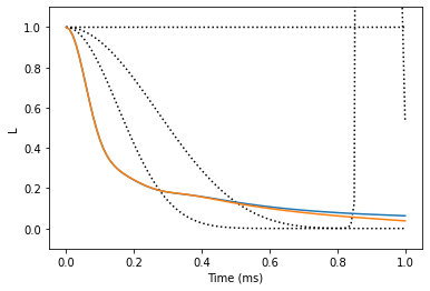
The gCCE results are converged at 1st order. Note that we used only a small number of bath states (30), thus the calculations are not converged with respect to the number of bath states. Calculations with higher number of bath states (~100) will produce correct results.
plt.plot(lgen, color='black', ls=':')
plt.plot(lgcce)

plt.xlabel('Time (ms)')
plt.ylabel('L')
plt.ylim(-0.1, 1.1);
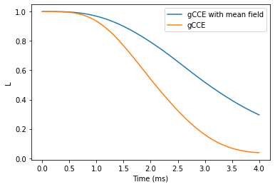
Hahn-echo decay
Using the similar procedure to the one used for FID, we can compute the Hahn-echo decay.
r_bath = 40
r_dipole = 8
order = 2
N = 1 # Number of pulses

calc = pc.Simulator(1, pos, bath=atoms, external_bath=exatoms,
                    pulses=N, D=D, E=E, alpha=-1, beta=0,
                    r_bath=r_bath, order=order, r_dipole=r_dipole)
ts = np.linspace(0, 4, 101) # time points (in ms)
helgen = calc.compute(ts, method='gcce', quantity='coherence')
Note the number of nbstates leads to significantly increased time of the calculation. The interface to mpi implementation is provided with keywords parallel (general) or parallel_states(bath state sampling run-specific). However it requires mpi4py installed and a run on several cores.
helgcce = calc.compute(time_space, nbstates=30, seed=seed,
                       method='gcce', quantity='coherence')
plt.plot(ts, helgcce, label='gCCE with mean field')
plt.plot(ts, helgen, label='gCCE')

plt.legend()
plt.xlabel('Time (ms)')
plt.ylabel('L');